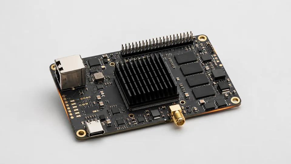
memory wall · edge LLM · LLM inference bandwidth · compute-in-memory · near-memory compute
The Memory Wall: Why Edge LLMs Stall and How to Get Around It
Fanshi Semiconductor engineering team · Published
The memory wall is the gap between fast-growing compute and slow-growing memory bandwidth, which leaves compute units waiting for data most of the time. In LLM decoding every token reads all of the weights, so the throughput ceiling equals memory bandwidth divided by model size. Edge devices have only tens of GB/s of bandwidth, so conventional architectures cannot run a capable LLM; compute-in-memory and near-memory compute get around the wall by moving weights less, or not at all.
One division
The decode throughput ceiling can be estimated with one division: tokens per second = memory bandwidth ÷ bytes of weights read per token. A 1B-parameter model at INT8 reads about 1 GB per token. On an edge device with 50 GB/s of bandwidth, the ceiling is 50 tokens per second, and that is the theoretical peak before real-world losses.
Switch to a 7B model and the same device manages about 7 tokens per second; at 35B, just over one. This is not a shortage of compute but a shortage of bandwidth. Adding TOPS changes nothing, because the compute units spend most of their time waiting for weights to arrive.
How data centres cope, and why edge devices cannot
The data-centre answer is HBM: several TB/s of bandwidth that enlarges the numerator. The price is hundreds of watts, thousands of dollars per accelerator and complex packaging. None of that works at the edge: handheld devices have a few watts, vehicles and robots a few tens of watts, and the silicon budget is measured in tens to hundreds of dollars.
So on conventional architectures, an edge LLM has two options: shrink the model drastically, or accept that it will be slow. Neither is attractive.
Getting around it: stop moving weights
Compute-in-memory builds multiply-accumulate into the memory array, so the weights take part in the computation where they sit and only activations travel on the bus. Activations are orders of magnitude smaller than the weights, so bandwidth stops being the bottleneck. MaskROM compute-in-memory goes furthest: the weights are cast into the silicon at tape-out, so even the read-out disappears.
Near-memory compute places the compute units right against high-bandwidth memory and uses on-chip streaming so that every weight read is fully reused, minimising both the number and the distance of transfers. It keeps the model updatable, which suits large models that are still evolving.
Both routes shrink the denominator of that division, or remove it, instead of brute-forcing a bigger numerator. That is why they can run edge LLMs on a mature 28 nm process.
What it means for products
Decode speed goes from a few tokens per second to more than ten thousand (design targets), so voice interaction no longer stalls and multi-stream workloads become possible. System power drops from over ten watts to the sub-watt class, so handheld devices can run offline all day. And without DRAM or HBM, both the BOM and the thermal design get simpler.
Fanshi Semiconductor's chips map onto the MaskROM, SRAM compute-in-memory and near-memory routes. To work out which one your product needs, start with "How to Choose an Edge LLM Inference Chip".